

Note
Click here to download the full example code
Introduces Gensim’s Word2Vec model and demonstrates its use on the Lee Corpus.
import logging
logging.basicConfig(format='%(asctime)s : %(levelname)s : %(message)s', level=logging.INFO)
In case you missed the buzz, word2vec is a widely featured as a member of the “new wave” of machine learning algorithms based on neural networks, commonly referred to as “deep learning” (though word2vec itself is rather shallow). Using large amounts of unannotated plain text, word2vec learns relationships between words automatically. The output are vectors, one vector per word, with remarkable linear relationships that allow us to do things like:
vec(“king”) - vec(“man”) + vec(“woman”) =~ vec(“queen”)
vec(“Montreal Canadiens”) – vec(“Montreal”) + vec(“Toronto”) =~ vec(“Toronto Maple Leafs”).
Word2vec is very useful in automatic text tagging, recommender systems and machine translation.
This tutorial:
Introduces Word2Vec as an improvement over traditional bag-of-words
Shows off a demo of Word2Vec using a pre-trained model
Demonstrates training a new model from your own data
Demonstrates loading and saving models
Introduces several training parameters and demonstrates their effect
Discusses memory requirements
Visualizes Word2Vec embeddings by applying dimensionality reduction
Note
Feel free to skip these review sections if you’re already familiar with the models.
You may be familiar with the bag-of-words model from the Vector section. This model transforms each document to a fixed-length vector of integers. For example, given the sentences:
John likes to watch movies. Mary likes movies too.
John also likes to watch football games. Mary hates football.
The model outputs the vectors:
[1, 2, 1, 1, 2, 1, 1, 0, 0, 0, 0]
[1, 1, 1, 1, 0, 1, 0, 1, 2, 1, 1]
Each vector has 10 elements, where each element counts the number of times a
particular word occurred in the document.
The order of elements is arbitrary.
In the example above, the order of the elements corresponds to the words:
["John", "likes", "to", "watch", "movies", "Mary", "too", "also", "football", "games", "hates"].
Bag-of-words models are surprisingly effective, but have several weaknesses.
First, they lose all information about word order: “John likes Mary” and “Mary likes John” correspond to identical vectors. There is a solution: bag of n-grams models consider word phrases of length n to represent documents as fixed-length vectors to capture local word order but suffer from data sparsity and high dimensionality.
Second, the model does not attempt to learn the meaning of the underlying
words, and as a consequence, the distance between vectors doesn’t always
reflect the difference in meaning. The Word2Vec model addresses this
second problem.
Word2Vec Model¶Word2Vec is a more recent model that embeds words in a lower-dimensional
vector space using a shallow neural network. The result is a set of
word-vectors where vectors close together in vector space have similar
meanings based on context, and word-vectors distant to each other have
differing meanings. For example, strong and powerful would be close
together and strong and Paris would be relatively far.
The are two versions of this model and Word2Vec
class implements them both:
Skip-grams (SG)
Continuous-bag-of-words (CBOW)
Important
Don’t let the implementation details below scare you. They’re advanced material: if it’s too much, then move on to the next section.
The Word2Vec Skip-gram model, for example, takes in pairs (word1, word2) generated by moving a window across text data, and trains a 1-hidden-layer neural network based on the synthetic task of given an input word, giving us a predicted probability distribution of nearby words to the input. A virtual one-hot encoding of words goes through a ‘projection layer’ to the hidden layer; these projection weights are later interpreted as the word embeddings. So if the hidden layer has 300 neurons, this network will give us 300-dimensional word embeddings.
Continuous-bag-of-words Word2vec is very similar to the skip-gram model. It is also a 1-hidden-layer neural network. The synthetic training task now uses the average of multiple input context words, rather than a single word as in skip-gram, to predict the center word. Again, the projection weights that turn one-hot words into averageable vectors, of the same width as the hidden layer, are interpreted as the word embeddings.
To see what Word2Vec can do, let’s download a pre-trained model and play
around with it. We will fetch the Word2Vec model trained on part of the
Google News dataset, covering approximately 3 million words and phrases. Such
a model can take hours to train, but since it’s already available,
downloading and loading it with Gensim takes minutes.
Important
The model is approximately 2GB, so you’ll need a decent network connection to proceed. Otherwise, skip ahead to the “Training Your Own Model” section below.
You may also check out an online word2vec demo where you can try
this vector algebra for yourself. That demo runs word2vec on the
entire Google News dataset, of about 100 billion words.
import gensim.downloader as api
wv = api.load('word2vec-google-news-300')
A common operation is to retrieve the vocabulary of a model. That is trivial:
for i, word in enumerate(wv.vocab):
    if i == 10:
        break
    print(word)
Out:
</s>
in
for
that
is
on
##
The
with
said
We can easily obtain vectors for terms the model is familiar with:
vec_king = wv['king']
Unfortunately, the model is unable to infer vectors for unfamiliar words. This is one limitation of Word2Vec: if this limitation matters to you, check out the FastText model.
try:
    vec_cameroon = wv['cameroon']
except KeyError:
    print("The word 'cameroon' does not appear in this model")
Out:
The word 'cameroon' does not appear in this model
Moving on, Word2Vec supports several word similarity tasks out of the
box. You can see how the similarity intuitively decreases as the words get
less and less similar.
pairs = [
    ('car', 'minivan'),   # a minivan is a kind of car
    ('car', 'bicycle'),   # still a wheeled vehicle
    ('car', 'airplane'),  # ok, no wheels, but still a vehicle
    ('car', 'cereal'),    # ... and so on
    ('car', 'communism'),
]
for w1, w2 in pairs:
    print('%r\t%r\t%.2f' % (w1, w2, wv.similarity(w1, w2)))
Out:
'car'   'minivan'       0.69
'car'   'bicycle'       0.54
'car'   'airplane'      0.42
'car'   'cereal'        0.14
'car'   'communism'     0.06
Print the 5 most similar words to “car” or “minivan”
print(wv.most_similar(positive=['car', 'minivan'], topn=5))
Out:
[('SUV', 0.853219211101532), ('vehicle', 0.8175784349441528), ('pickup_truck', 0.7763689160346985), ('Jeep', 0.7567334175109863), ('Ford_Explorer', 0.756571888923645)]
Which of the below does not belong in the sequence?
print(wv.doesnt_match(['fire', 'water', 'land', 'sea', 'air', 'car']))
Out:
/home/misha/git/gensim/gensim/models/keyedvectors.py:877: FutureWarning: arrays to stack must be passed as a "sequence" type such as list or tuple. Support for non-sequence iterables such as generators is deprecated as of NumPy 1.16 and will raise an error in the future.
  vectors = vstack(self.word_vec(word, use_norm=True) for word in used_words).astype(REAL)
car
To start, you’ll need some data for training the model. For the following examples, we’ll use the Lee Corpus (which you already have if you’ve installed gensim).
This corpus is small enough to fit entirely in memory, but we’ll implement a memory-friendly iterator that reads it line-by-line to demonstrate how you would handle a larger corpus.
from gensim.test.utils import datapath
from gensim import utils

class MyCorpus(object):
    """An interator that yields sentences (lists of str)."""

    def __iter__(self):
        corpus_path = datapath('lee_background.cor')
        for line in open(corpus_path):
            # assume there's one document per line, tokens separated by whitespace
            yield utils.simple_preprocess(line)
If we wanted to do any custom preprocessing, e.g. decode a non-standard
encoding, lowercase, remove numbers, extract named entities… All of this can
be done inside the MyCorpus iterator and word2vec doesn’t need to
know. All that is required is that the input yields one sentence (list of
utf8 words) after another.
Let’s go ahead and train a model on our corpus. Don’t worry about the training parameters much for now, we’ll revisit them later.
import gensim.models

sentences = MyCorpus()
model = gensim.models.Word2Vec(sentences=sentences)
Once we have our model, we can use it in the same way as in the demo above.
The main part of the model is model.wv, where “wv” stands for “word vectors”.
vec_king = model.wv['king']
Retrieving the vocabulary works the same way:
for i, word in enumerate(model.wv.vocab):
    if i == 10:
        break
    print(word)
Out:
hundreds
of
people
have
been
forced
to
their
homes
in
You’ll notice that training non-trivial models can take time. Once you’ve trained your model and it works as expected, you can save it to disk. That way, you don’t have to spend time training it all over again later.
You can store/load models using the standard gensim methods:
import tempfile

with tempfile.NamedTemporaryFile(prefix='gensim-model-', delete=False) as tmp:
    temporary_filepath = tmp.name
    model.save(temporary_filepath)
    #
    # The model is now safely stored in the filepath.
    # You can copy it to other machines, share it with others, etc.
    #
    # To load a saved model:
    #
    new_model = gensim.models.Word2Vec.load(temporary_filepath)
which uses pickle internally, optionally mmap‘ing the model’s internal
large NumPy matrices into virtual memory directly from disk files, for
inter-process memory sharing.
In addition, you can load models created by the original C tool, both using its text and binary formats:
model = gensim.models.KeyedVectors.load_word2vec_format('/tmp/vectors.txt', binary=False)
# using gzipped/bz2 input works too, no need to unzip
model = gensim.models.KeyedVectors.load_word2vec_format('/tmp/vectors.bin.gz', binary=True)
Word2Vec accepts several parameters that affect both training speed and quality.
min_count is for pruning the internal dictionary. Words that appear only
once or twice in a billion-word corpus are probably uninteresting typos and
garbage. In addition, there’s not enough data to make any meaningful training
on those words, so it’s best to ignore them:
default value of min_count=5
model = gensim.models.Word2Vec(sentences, min_count=10)
size is the number of dimensions (N) of the N-dimensional space that
gensim Word2Vec maps the words onto.
Bigger size values require more training data, but can lead to better (more accurate) models. Reasonable values are in the tens to hundreds.
# default value of size=100
model = gensim.models.Word2Vec(sentences, size=200)
workers , the last of the major parameters (full list here)
is for training parallelization, to speed up training:
# default value of workers=3 (tutorial says 1...)
model = gensim.models.Word2Vec(sentences, workers=4)
The workers parameter only has an effect if you have Cython installed. Without Cython, you’ll only be able to use
one core because of the GIL (and word2vec
training will be miserably slow).
At its core, word2vec model parameters are stored as matrices (NumPy
arrays). Each array is #vocabulary (controlled by min_count parameter)
times #size (size parameter) of floats (single precision aka 4 bytes).
Three such matrices are held in RAM (work is underway to reduce that number
to two, or even one). So if your input contains 100,000 unique words, and you
asked for layer size=200, the model will require approx.
100,000*200*4*3 bytes = ~229MB.
There’s a little extra memory needed for storing the vocabulary tree (100,000 words would take a few megabytes), but unless your words are extremely loooong strings, memory footprint will be dominated by the three matrices above.
Word2Vec training is an unsupervised task, there’s no good way to
objectively evaluate the result. Evaluation depends on your end application.
Google has released their testing set of about 20,000 syntactic and semantic test examples, following the “A is to B as C is to D” task. It is provided in the ‘datasets’ folder.
For example a syntactic analogy of comparative type is bad:worse;good:?. There are total of 9 types of syntactic comparisons in the dataset like plural nouns and nouns of opposite meaning.
The semantic questions contain five types of semantic analogies, such as capital cities (Paris:France;Tokyo:?) or family members (brother:sister;dad:?).
Gensim supports the same evaluation set, in exactly the same format:
model.accuracy('./datasets/questions-words.txt')
This accuracy takes an optional parameter
restrict_vocab which limits which test examples are to be considered.
In the December 2016 release of Gensim we added a better way to evaluate semantic similarity.
By default it uses an academic dataset WS-353 but one can create a dataset specific to your business based on it. It contains word pairs together with human-assigned similarity judgments. It measures the relatedness or co-occurrence of two words. For example, ‘coast’ and ‘shore’ are very similar as they appear in the same context. At the same time ‘clothes’ and ‘closet’ are less similar because they are related but not interchangeable.
model.evaluate_word_pairs(datapath('wordsim353.tsv'))
Important
Good performance on Google’s or WS-353 test set doesn’t mean word2vec will work well in your application, or vice versa. It’s always best to evaluate directly on your intended task. For an example of how to use word2vec in a classifier pipeline, see this tutorial.
Advanced users can load a model and continue training it with more sentences and new vocabulary words:
model = gensim.models.Word2Vec.load(temporary_filepath)
more_sentences = [
    ['Advanced', 'users', 'can', 'load', 'a', 'model',
     'and', 'continue', 'training', 'it', 'with', 'more', 'sentences']
]
model.build_vocab(more_sentences, update=True)
model.train(more_sentences, total_examples=model.corpus_count, epochs=model.iter)

# cleaning up temporary file
import os
os.remove(temporary_filepath)
You may need to tweak the total_words parameter to train(),
depending on what learning rate decay you want to simulate.
Note that it’s not possible to resume training with models generated by the C
tool, KeyedVectors.load_word2vec_format(). You can still use them for
querying/similarity, but information vital for training (the vocab tree) is
missing there.
The parameter compute_loss can be used to toggle computation of loss
while training the Word2Vec model. The computed loss is stored in the model
attribute running_training_loss and can be retrieved using the function
get_latest_training_loss as follows :
# instantiating and training the Word2Vec model
model_with_loss = gensim.models.Word2Vec(
    sentences,
    min_count=1,
    compute_loss=True,
    hs=0,
    sg=1,
    seed=42
)

# getting the training loss value
training_loss = model_with_loss.get_latest_training_loss()
print(training_loss)
Out:
1376815.375
Let’s run some benchmarks to see effect of the training loss computation code on training time.
We’ll use the following data for the benchmarks:
Lee Background corpus: included in gensim’s test data
Text8 corpus. To demonstrate the effect of corpus size, we’ll look at the first 1MB, 10MB, 50MB of the corpus, as well as the entire thing.
import io
import os

import gensim.models.word2vec
import gensim.downloader as api
import smart_open


def head(path, size):
    with smart_open.open(path) as fin:
        return io.StringIO(fin.read(size))


def generate_input_data():
    lee_path = datapath('lee_background.cor')
    ls = gensim.models.word2vec.LineSentence(lee_path)
    ls.name = '25kB'
    yield ls

    text8_path = api.load('text8').fn
    labels = ('1MB', '10MB', '50MB', '100MB')
    sizes = (1024 ** 2, 10 * 1024 ** 2, 50 * 1024 ** 2, 100 * 1024 ** 2)
    for l, s in zip(labels, sizes):
        ls = gensim.models.word2vec.LineSentence(head(text8_path, s))
        ls.name = l
        yield ls


input_data = list(generate_input_data())
We now compare the training time taken for different combinations of input
data and model training parameters like hs and sg.
For each combination, we repeat the test several times to obtain the mean and standard deviation of the test duration.
# Temporarily reduce logging verbosity
logging.root.level = logging.ERROR

import time
import numpy as np
import pandas as pd

train_time_values = []
seed_val = 42
sg_values = [0, 1]
hs_values = [0, 1]

fast = True
if fast:
    input_data_subset = input_data[:3]
else:
    input_data_subset = input_data


for data in input_data_subset:
    for sg_val in sg_values:
        for hs_val in hs_values:
            for loss_flag in [True, False]:
                time_taken_list = []
                for i in range(3):
                    start_time = time.time()
                    w2v_model = gensim.models.Word2Vec(
                        data,
                        compute_loss=loss_flag,
                        sg=sg_val,
                        hs=hs_val,
                        seed=seed_val,
                    )
                    time_taken_list.append(time.time() - start_time)

                time_taken_list = np.array(time_taken_list)
                time_mean = np.mean(time_taken_list)
                time_std = np.std(time_taken_list)

                model_result = {
                    'train_data': data.name,
                    'compute_loss': loss_flag,
                    'sg': sg_val,
                    'hs': hs_val,
                    'train_time_mean': time_mean,
                    'train_time_std': time_std,
                }
                print("Word2vec model #%i: %s" % (len(train_time_values), model_result))
                train_time_values.append(model_result)

train_times_table = pd.DataFrame(train_time_values)
train_times_table = train_times_table.sort_values(
    by=['train_data', 'sg', 'hs', 'compute_loss'],
    ascending=[False, False, True, False],
)
print(train_times_table)
Out:
Word2vec model #0: {'train_data': '25kB', 'compute_loss': True, 'sg': 0, 'hs': 0, 'train_time_mean': 0.42024485270182294, 'train_time_std': 0.010698776849185184}
Word2vec model #1: {'train_data': '25kB', 'compute_loss': False, 'sg': 0, 'hs': 0, 'train_time_mean': 0.4227687517801921, 'train_time_std': 0.010170030330566043}
Word2vec model #2: {'train_data': '25kB', 'compute_loss': True, 'sg': 0, 'hs': 1, 'train_time_mean': 0.536113421122233, 'train_time_std': 0.004805753793586722}
Word2vec model #3: {'train_data': '25kB', 'compute_loss': False, 'sg': 0, 'hs': 1, 'train_time_mean': 0.5387027263641357, 'train_time_std': 0.008667062182886069}
Word2vec model #4: {'train_data': '25kB', 'compute_loss': True, 'sg': 1, 'hs': 0, 'train_time_mean': 0.6562980810801188, 'train_time_std': 0.013588778726591642}
Word2vec model #5: {'train_data': '25kB', 'compute_loss': False, 'sg': 1, 'hs': 0, 'train_time_mean': 0.6652247111002604, 'train_time_std': 0.011507952438692074}
Word2vec model #6: {'train_data': '25kB', 'compute_loss': True, 'sg': 1, 'hs': 1, 'train_time_mean': 1.063435713450114, 'train_time_std': 0.007722866080141013}
Word2vec model #7: {'train_data': '25kB', 'compute_loss': False, 'sg': 1, 'hs': 1, 'train_time_mean': 1.0656228065490723, 'train_time_std': 0.010417429290681622}
Word2vec model #8: {'train_data': '1MB', 'compute_loss': True, 'sg': 0, 'hs': 0, 'train_time_mean': 1.1557533740997314, 'train_time_std': 0.021498065208364548}
Word2vec model #9: {'train_data': '1MB', 'compute_loss': False, 'sg': 0, 'hs': 0, 'train_time_mean': 1.1348456541697185, 'train_time_std': 0.008478234726085157}
Word2vec model #10: {'train_data': '1MB', 'compute_loss': True, 'sg': 0, 'hs': 1, 'train_time_mean': 1.5982224941253662, 'train_time_std': 0.032441277082374986}
Word2vec model #11: {'train_data': '1MB', 'compute_loss': False, 'sg': 0, 'hs': 1, 'train_time_mean': 1.6024325688680012, 'train_time_std': 0.05484816962039394}
Word2vec model #12: {'train_data': '1MB', 'compute_loss': True, 'sg': 1, 'hs': 0, 'train_time_mean': 2.0538527170817056, 'train_time_std': 0.02116566035017678}
Word2vec model #13: {'train_data': '1MB', 'compute_loss': False, 'sg': 1, 'hs': 0, 'train_time_mean': 2.095852772394816, 'train_time_std': 0.027719772722993145}
Word2vec model #14: {'train_data': '1MB', 'compute_loss': True, 'sg': 1, 'hs': 1, 'train_time_mean': 3.8532145023345947, 'train_time_std': 0.13194007715689138}
Word2vec model #15: {'train_data': '1MB', 'compute_loss': False, 'sg': 1, 'hs': 1, 'train_time_mean': 4.347004095713298, 'train_time_std': 0.4074951861350163}
Word2vec model #16: {'train_data': '10MB', 'compute_loss': True, 'sg': 0, 'hs': 0, 'train_time_mean': 9.744145313898722, 'train_time_std': 0.528574777917741}
Word2vec model #17: {'train_data': '10MB', 'compute_loss': False, 'sg': 0, 'hs': 0, 'train_time_mean': 10.102657397588095, 'train_time_std': 0.04922284567998143}
Word2vec model #18: {'train_data': '10MB', 'compute_loss': True, 'sg': 0, 'hs': 1, 'train_time_mean': 14.720670620600382, 'train_time_std': 0.14477234755034}
Word2vec model #19: {'train_data': '10MB', 'compute_loss': False, 'sg': 0, 'hs': 1, 'train_time_mean': 15.064472993214926, 'train_time_std': 0.13933597618834875}
Word2vec model #20: {'train_data': '10MB', 'compute_loss': True, 'sg': 1, 'hs': 0, 'train_time_mean': 22.98580002784729, 'train_time_std': 0.13657929022316737}
Word2vec model #21: {'train_data': '10MB', 'compute_loss': False, 'sg': 1, 'hs': 0, 'train_time_mean': 22.99385412534078, 'train_time_std': 0.4251254084886872}
Word2vec model #22: {'train_data': '10MB', 'compute_loss': True, 'sg': 1, 'hs': 1, 'train_time_mean': 43.337499936421715, 'train_time_std': 0.8026425548453814}
Word2vec model #23: {'train_data': '10MB', 'compute_loss': False, 'sg': 1, 'hs': 1, 'train_time_mean': 41.70925132433573, 'train_time_std': 0.2547404428238225}
   train_data  compute_loss  sg  hs  train_time_mean  train_time_std
4        25kB          True   1   0         0.656298        0.013589
5        25kB         False   1   0         0.665225        0.011508
6        25kB          True   1   1         1.063436        0.007723
7        25kB         False   1   1         1.065623        0.010417
0        25kB          True   0   0         0.420245        0.010699
1        25kB         False   0   0         0.422769        0.010170
2        25kB          True   0   1         0.536113        0.004806
3        25kB         False   0   1         0.538703        0.008667
12        1MB          True   1   0         2.053853        0.021166
13        1MB         False   1   0         2.095853        0.027720
14        1MB          True   1   1         3.853215        0.131940
15        1MB         False   1   1         4.347004        0.407495
8         1MB          True   0   0         1.155753        0.021498
9         1MB         False   0   0         1.134846        0.008478
10        1MB          True   0   1         1.598222        0.032441
11        1MB         False   0   1         1.602433        0.054848
20       10MB          True   1   0        22.985800        0.136579
21       10MB         False   1   0        22.993854        0.425125
22       10MB          True   1   1        43.337500        0.802643
23       10MB         False   1   1        41.709251        0.254740
16       10MB          True   0   0         9.744145        0.528575
17       10MB         False   0   0        10.102657        0.049223
18       10MB          True   0   1        14.720671        0.144772
19       10MB         False   0   1        15.064473        0.139336
Suppose, we still want more performance improvement in production.
One good way is to cache all the similar words in a dictionary.
So that next time when we get the similar query word, we’ll search it first in the dict.
And if it’s a hit then we will show the result directly from the dictionary.
otherwise we will query the word and then cache it so that it doesn’t miss next time.
# re-enable logging
logging.root.level = logging.INFO

most_similars_precalc = {word : model.wv.most_similar(word) for word in model.wv.index2word}
for i, (key, value) in enumerate(most_similars_precalc.items()):
    if i == 3:
        break
    print(key, value)
Out:
the [('of', 0.999931812286377), ('at', 0.999925434589386), ('state', 0.9999253153800964), ('and', 0.9999250769615173), ('from', 0.9999250173568726), ('world', 0.9999234676361084), ('its', 0.9999232292175293), ('first', 0.9999232292175293), ('australia', 0.9999231100082397), ('one', 0.9999231100082397)]
to [('at', 0.999946117401123), ('if', 0.9999457597732544), ('will', 0.9999451637268066), ('out', 0.9999433159828186), ('or', 0.999942421913147), ('are', 0.9999421238899231), ('that', 0.9999387264251709), ('but', 0.9999367594718933), ('into', 0.999936580657959), ('from', 0.9999353885650635)]
of [('first', 0.9999472498893738), ('at', 0.999944806098938), ('australian', 0.9999432563781738), ('into', 0.9999418258666992), ('three', 0.9999409914016724), ('with', 0.999938428401947), ('over', 0.9999372363090515), ('in', 0.9999370574951172), ('by', 0.9999368786811829), ('and', 0.9999358654022217)]
for time being lets take 4 words randomly
import time
words = ['voted', 'few', 'their', 'around']
Without caching
start = time.time()
for word in words:
    result = model.wv.most_similar(word)
    print(result)
end = time.time()
print(end - start)
Out:
[('flights', 0.9986665844917297), ('job', 0.9986284971237183), ('building', 0.9985975623130798), ('see', 0.9985952377319336), ('figures', 0.9985781311988831), ('melbourne', 0.9985730051994324), ('two', 0.9985727071762085), ('per', 0.9985710978507996), ('weather', 0.9985674619674683), ('still', 0.9985595345497131)]
[('an', 0.9997475147247314), ('today', 0.999739408493042), ('were', 0.9997352361679077), ('after', 0.9997317790985107), ('which', 0.9997289180755615), ('with', 0.9997268915176392), ('against', 0.999722957611084), ('still', 0.9997221231460571), ('at', 0.9997204542160034), ('could', 0.9997197389602661)]
[('at', 0.9999508857727051), ('from', 0.9999468326568604), ('up', 0.9999455809593201), ('today', 0.9999449849128723), ('us', 0.9999443292617798), ('on', 0.999944269657135), ('his', 0.9999438524246216), ('by', 0.9999434947967529), ('into', 0.9999425411224365), ('with', 0.9999420642852783)]
[('by', 0.9999364018440247), ('out', 0.999934732913971), ('after', 0.9999337196350098), ('into', 0.9999316334724426), ('at', 0.9999312162399292), ('and', 0.9999300241470337), ('with', 0.9999291896820068), ('over', 0.9999289512634277), ('as', 0.9999284744262695), ('were', 0.9999282360076904)]
0.030631542205810547
Now with caching
start = time.time()
for word in words:
    if 'voted' in most_similars_precalc:
        result = most_similars_precalc[word]
        print(result)
    else:
        result = model.wv.most_similar(word)
        most_similars_precalc[word] = result
        print(result)

end = time.time()
print(end - start)
Out:
[('flights', 0.9986665844917297), ('job', 0.9986284971237183), ('building', 0.9985975623130798), ('see', 0.9985952377319336), ('figures', 0.9985781311988831), ('melbourne', 0.9985730051994324), ('two', 0.9985727071762085), ('per', 0.9985710978507996), ('weather', 0.9985674619674683), ('still', 0.9985595345497131)]
[('an', 0.9997475147247314), ('today', 0.999739408493042), ('were', 0.9997352361679077), ('after', 0.9997317790985107), ('which', 0.9997289180755615), ('with', 0.9997268915176392), ('against', 0.999722957611084), ('still', 0.9997221231460571), ('at', 0.9997204542160034), ('could', 0.9997197389602661)]
[('at', 0.9999508857727051), ('from', 0.9999468326568604), ('up', 0.9999455809593201), ('today', 0.9999449849128723), ('us', 0.9999443292617798), ('on', 0.999944269657135), ('his', 0.9999438524246216), ('by', 0.9999434947967529), ('into', 0.9999425411224365), ('with', 0.9999420642852783)]
[('by', 0.9999364018440247), ('out', 0.999934732913971), ('after', 0.9999337196350098), ('into', 0.9999316334724426), ('at', 0.9999312162399292), ('and', 0.9999300241470337), ('with', 0.9999291896820068), ('over', 0.9999289512634277), ('as', 0.9999284744262695), ('were', 0.9999282360076904)]
0.0009360313415527344
Clearly you can see the improvement but this difference will be even larger when we take more words in the consideration.
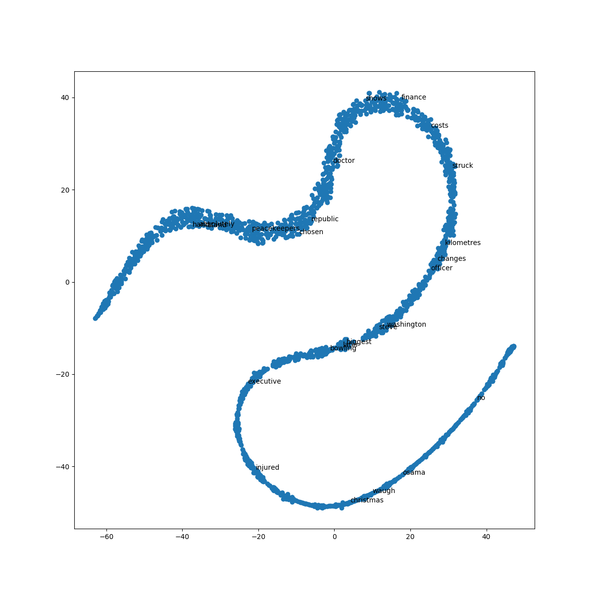
The word embeddings made by the model can be visualised by reducing dimensionality of the words to 2 dimensions using tSNE.
Visualisations can be used to notice semantic and syntactic trends in the data.
Example:
Semantic: words like cat, dog, cow, etc. have a tendency to lie close by
Syntactic: words like run, running or cut, cutting lie close together.
Vector relations like vKing - vMan = vQueen - vWoman can also be noticed.
Important
The model used for the visualisation is trained on a small corpus. Thus some of the relations might not be so clear.
from sklearn.decomposition import IncrementalPCA    # inital reduction
from sklearn.manifold import TSNE                   # final reduction
import numpy as np                                  # array handling


def reduce_dimensions(model):
    num_dimensions = 2  # final num dimensions (2D, 3D, etc)

    vectors = [] # positions in vector space
    labels = [] # keep track of words to label our data again later
    for word in model.wv.vocab:
        vectors.append(model.wv[word])
        labels.append(word)

    # convert both lists into numpy vectors for reduction
    vectors = np.asarray(vectors)
    labels = np.asarray(labels)

    # reduce using t-SNE
    vectors = np.asarray(vectors)
    tsne = TSNE(n_components=num_dimensions, random_state=0)
    vectors = tsne.fit_transform(vectors)

    x_vals = [v[0] for v in vectors]
    y_vals = [v[1] for v in vectors]
    return x_vals, y_vals, labels


x_vals, y_vals, labels = reduce_dimensions(model)

def plot_with_plotly(x_vals, y_vals, labels, plot_in_notebook=True):
    from plotly.offline import init_notebook_mode, iplot, plot
    import plotly.graph_objs as go

    trace = go.Scatter(x=x_vals, y=y_vals, mode='text', text=labels)
    data = [trace]

    if plot_in_notebook:
        init_notebook_mode(connected=True)
        iplot(data, filename='word-embedding-plot')
    else:
        plot(data, filename='word-embedding-plot.html')


def plot_with_matplotlib(x_vals, y_vals, labels):
    import matplotlib.pyplot as plt
    import random

    random.seed(0)

    plt.figure(figsize=(12, 12))
    plt.scatter(x_vals, y_vals)

    #
    # Label randomly subsampled 25 data points
    #
    indices = list(range(len(labels)))
    selected_indices = random.sample(indices, 25)
    for i in selected_indices:
        plt.annotate(labels[i], (x_vals[i], y_vals[i]))

try:
    get_ipython()
except Exception:
    plot_function = plot_with_matplotlib
else:
    plot_function = plot_with_plotly

plot_function(x_vals, y_vals, labels)
In this tutorial we learned how to train word2vec models on your custom data and also how to evaluate it. Hope that you too will find this popular tool useful in your Machine Learning tasks!
Total running time of the script: ( 14 minutes 57.464 seconds)
Estimated memory usage: 11388 MB
