How to Compare LDA Models

How to Compare LDA Models

Demonstrates how you can compare a topic model with itself or other models.

# sphinx_gallery_thumbnail_number = 2
import logging
logging.basicConfig(format='%(asctime)s : %(levelname)s : %(message)s', level=logging.INFO)

First, clean up the 20 Newsgroups dataset. We will use it to fit LDA.

from string import punctuation
from nltk import RegexpTokenizer
from nltk.stem.porter import PorterStemmer
from nltk.corpus import stopwords
from sklearn.datasets import fetch_20newsgroups


newsgroups = fetch_20newsgroups()
eng_stopwords = set(stopwords.words('english'))

tokenizer = RegexpTokenizer(r'\s+', gaps=True)
stemmer = PorterStemmer()
translate_tab = {ord(p): u" " for p in punctuation}

def text2tokens(raw_text):
    """Convert a raw text to a list of stemmed tokens."""
    clean_text = raw_text.lower().translate(translate_tab)
    tokens = [token.strip() for token in tokenizer.tokenize(clean_text)]
    tokens = [token for token in tokens if token not in eng_stopwords]
    stemmed_tokens = [stemmer.stem(token) for token in tokens]
    return [token for token in stemmed_tokens if len(token) > 2]  # skip short tokens

dataset = [text2tokens(txt) for txt in newsgroups['data']]  # convert a documents to list of tokens

from gensim.corpora import Dictionary
dictionary = Dictionary(documents=dataset, prune_at=None)
dictionary.filter_extremes(no_below=5, no_above=0.3, keep_n=None)  # use Dictionary to remove un-relevant tokens
dictionary.compactify()

d2b_dataset = [dictionary.doc2bow(doc) for doc in dataset]  # convert list of tokens to bag of word representation

Second, fit two LDA models.

from gensim.models import LdaMulticore
num_topics = 15

lda_fst = LdaMulticore(
    corpus=d2b_dataset, num_topics=num_topics, id2word=dictionary,
    workers=4, eval_every=None, passes=10, batch=True
)

lda_snd = LdaMulticore(
    corpus=d2b_dataset, num_topics=num_topics, id2word=dictionary,
    workers=4, eval_every=None, passes=20, batch=True
)

Time to visualize, yay!

We use two slightly different visualization methods depending on how you’re running this tutorial. If you’re running via a Jupyter notebook, then you’ll get a nice interactive Plotly heatmap. If you’re viewing the static version of the page, you’ll get a similar matplotlib heatmap, but it won’t be interactive.

def plot_difference_plotly(mdiff, title="", annotation=None):
    """Plot the difference between models.

    Uses plotly as the backend."""
    import plotly.graph_objs as go
    import plotly.offline as py

    annotation_html = None
    if annotation is not None:
        annotation_html = [
            [
                "+++ {}<br>--- {}".format(", ".join(int_tokens), ", ".join(diff_tokens))
                for (int_tokens, diff_tokens) in row
            ]
            for row in annotation
        ]

    data = go.Heatmap(z=mdiff, colorscale='RdBu', text=annotation_html)
    layout = go.Layout(width=950, height=950, title=title, xaxis=dict(title="topic"), yaxis=dict(title="topic"))
    py.iplot(dict(data=[data], layout=layout))


def plot_difference_matplotlib(mdiff, title="", annotation=None):
    """Helper function to plot difference between models.

    Uses matplotlib as the backend."""
    import matplotlib.pyplot as plt
    fig, ax = plt.subplots(figsize=(18, 14))
    data = ax.imshow(mdiff, cmap='RdBu_r', origin='lower')
    plt.title(title)
    plt.colorbar(data)


try:
    get_ipython()
    import plotly.offline as py
except Exception:
    #
    # Fall back to matplotlib if we're not in a notebook, or if plotly is
    # unavailable for whatever reason.
    #
    plot_difference = plot_difference_matplotlib
else:
    py.init_notebook_mode()
    plot_difference = plot_difference_plotly

Gensim can help you visualise the differences between topics. For this purpose, you can use the diff() method of LdaModel.

diff() returns a matrix with distances mdiff and a matrix with annotations annotation. Read the docstring for more detailed info.

In each mdiff[i][j] cell you’ll find a distance between topic_i from the first model and topic_j from the second model.

In each annotation[i][j] cell you’ll find [tokens from intersection, tokens from difference between topic_i from first model and topic_j from the second model.

print(LdaMulticore.diff.__doc__)

Out:

Calculate the difference in topic distributions between two models: `self` and `other`.

        Parameters
        ----------
        other : :class:`~gensim.models.ldamodel.LdaModel`
            The model which will be compared against the current object.
        distance : {'kullback_leibler', 'hellinger', 'jaccard', 'jensen_shannon'}
            The distance metric to calculate the difference with.
        num_words : int, optional
            The number of most relevant words used if `distance == 'jaccard'`. Also used for annotating topics.
        n_ann_terms : int, optional
            Max number of words in intersection/symmetric difference between topics. Used for annotation.
        diagonal : bool, optional
            Whether we need the difference between identical topics (the diagonal of the difference matrix).
        annotation : bool, optional
            Whether the intersection or difference of words between two topics should be returned.
        normed : bool, optional
            Whether the matrix should be normalized or not.

        Returns
        -------
        numpy.ndarray
            A difference matrix. Each element corresponds to the difference between the two topics,
            shape (`self.num_topics`, `other.num_topics`)
        numpy.ndarray, optional
            Annotation matrix where for each pair we include the word from the intersection of the two topics,
            and the word from the symmetric difference of the two topics. Only included if `annotation == True`.
            Shape (`self.num_topics`, `other_model.num_topics`, 2).

        Examples
        --------
        Get the differences between each pair of topics inferred by two models

        .. sourcecode:: pycon

            >>> from gensim.models.ldamulticore import LdaMulticore
            >>> from gensim.test.utils import datapath
            >>>
            >>> m1 = LdaMulticore.load(datapath("lda_3_0_1_model"))
            >>> m2 = LdaMulticore.load(datapath("ldamodel_python_3_5"))
            >>> mdiff, annotation = m1.diff(m2)
            >>> topic_diff = mdiff  # get matrix with difference for each topic pair from `m1` and `m2`

Case 1: How topics within ONE model correlate with each other.

Short description:

• x-axis - topic;

• y-axis - topic;

• almost red cell - strongly decorrelated topics;

• almost blue cell - strongly correlated topics.

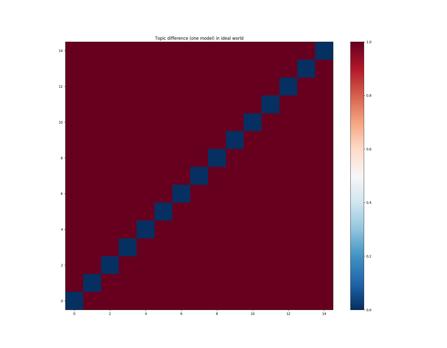
In an ideal world, we would like to see different topics decorrelated between themselves. In this case, our matrix would look like this:

import numpy as np

mdiff = np.ones((num_topics, num_topics))
np.fill_diagonal(mdiff, 0.)
plot_difference(mdiff, title="Topic difference (one model) in ideal world")

Unfortunately, in real life, not everything is so good, and the matrix looks different.

Short description (interactive annotations only):

• +++ make, world, well - words from the intersection of topics = present in both topics;

• --- money, day, still - words from the symmetric difference of topics = present in one topic but not the other.

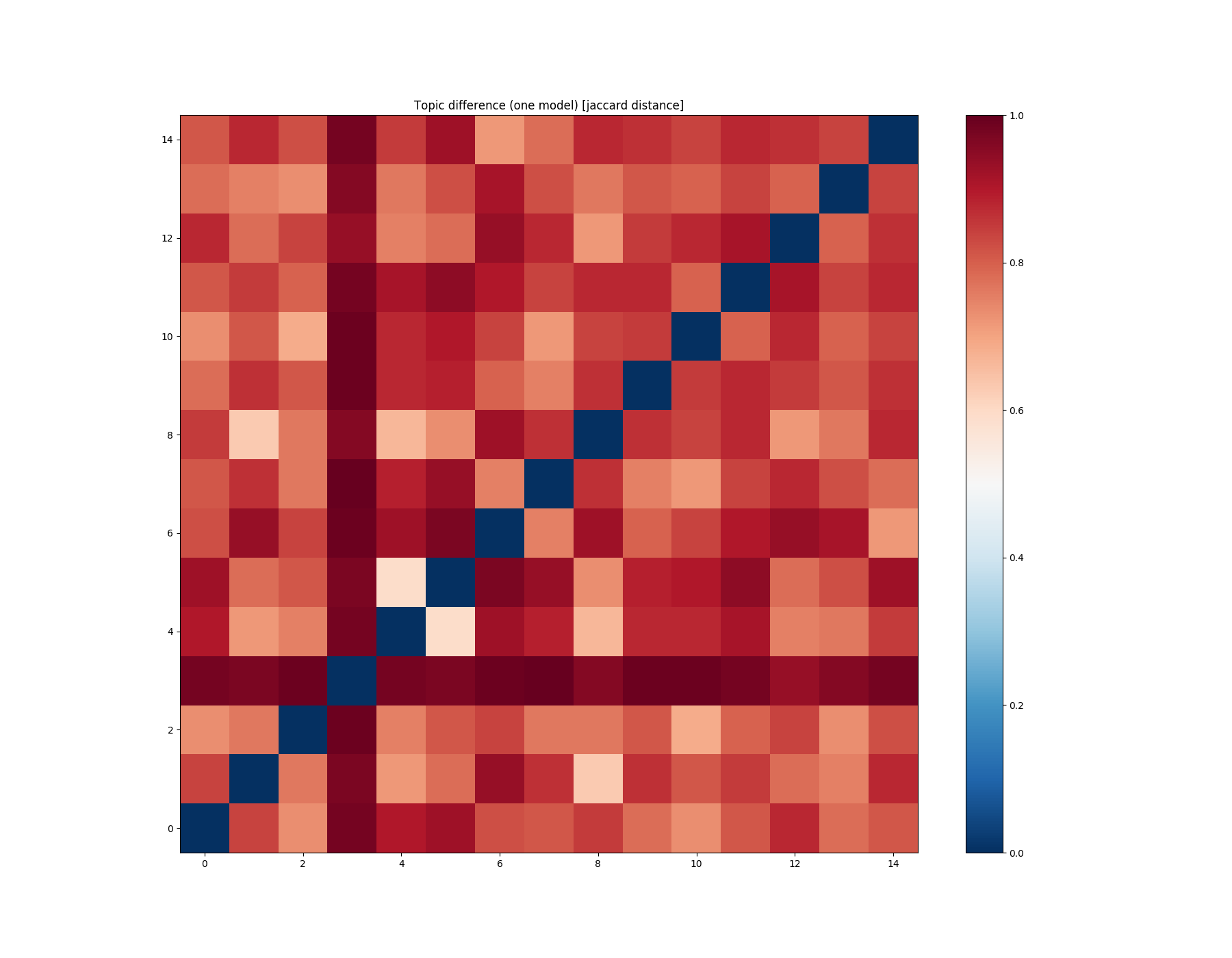
mdiff, annotation = lda_fst.diff(lda_fst, distance='jaccard', num_words=50)
plot_difference(mdiff, title="Topic difference (one model) [jaccard distance]", annotation=annotation)

If you compare a model with itself, you want to see as many red elements as possible (except diagonal). With this picture, you can look at the not very red elements and understand which topics in the model are very similar and why (you can read annotation if you move your pointer to cell).

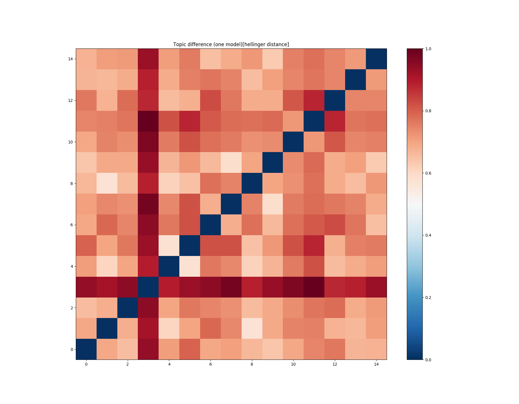
Jaccard is stable and robust distance function, but this function not enough sensitive for some purposes. Let’s try to use Hellinger distance now.

mdiff, annotation = lda_fst.diff(lda_fst, distance='hellinger', num_words=50)
plot_difference(mdiff, title="Topic difference (one model)[hellinger distance]", annotation=annotation)

You see that everything has become worse, but remember that everything depends on the task.

You need to choose the function with which your personal point of view about topics similarity and your task (from my experience, Jaccard is fine).

Case 2: How topics from DIFFERENT models correlate with each other.

Sometimes, we want to look at the patterns between two different models and compare them.

You can do this by constructing a matrix with the difference.

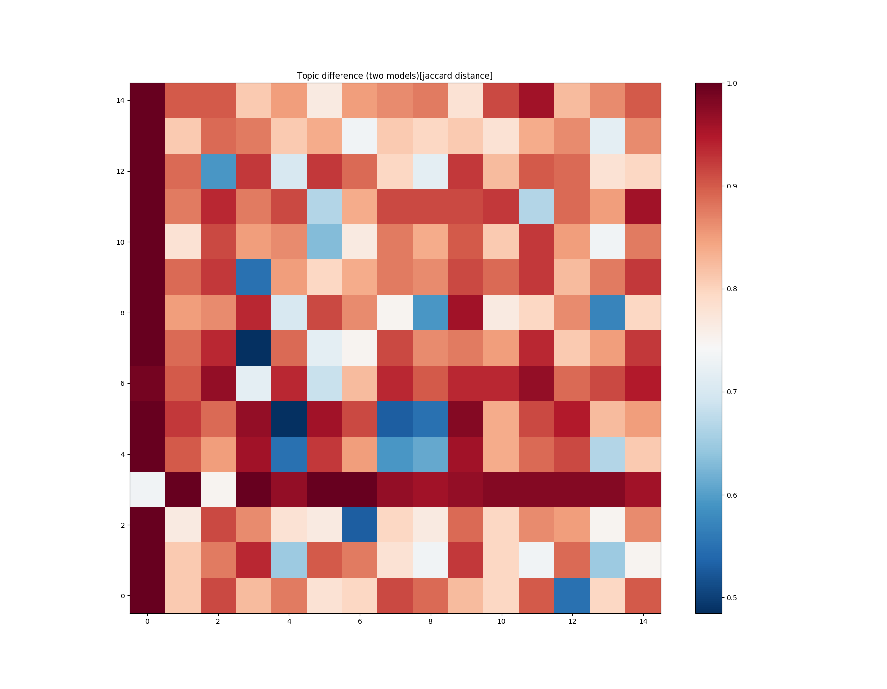
mdiff, annotation = lda_fst.diff(lda_snd, distance='jaccard', num_words=50)
plot_difference(mdiff, title="Topic difference (two models)[jaccard distance]", annotation=annotation)

Looking at this matrix, you can find similar and different topics (and relevant tokens which describe the intersection and difference).

Estimated memory usage: 389 MB