 RARE Technologies
Previous posts explained the whys & whats of nearest-neighbour search, the available OSS libraries and Python wrappers. We converted the English Wikipedia to vector space, to be used as our testing dataset for retrieving “similar articles”. In this post, I finally get to some hard performance numbers, plus a live demo near the end.
Accuracy
First, there’s an obvious tradeoff between accuracy and performance — the approximation methods can be as fast as you like, as long as you don’t mind them returning rubbish. So I’ll be scatter-plotting speed vs. accuracy in a single graph, like for FLANN here:
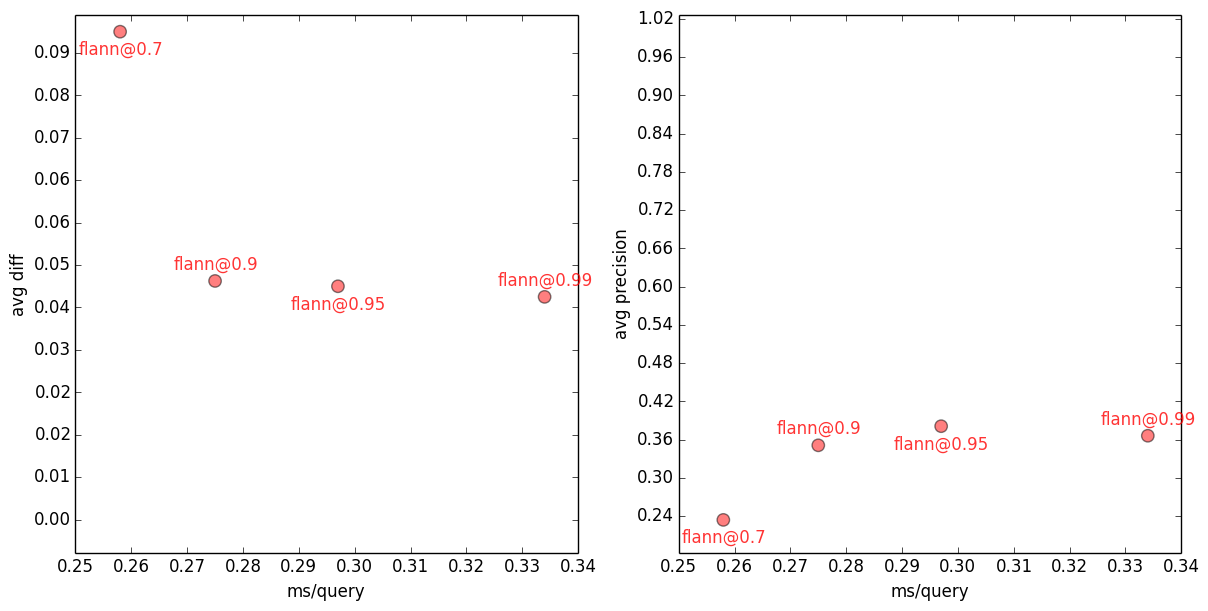
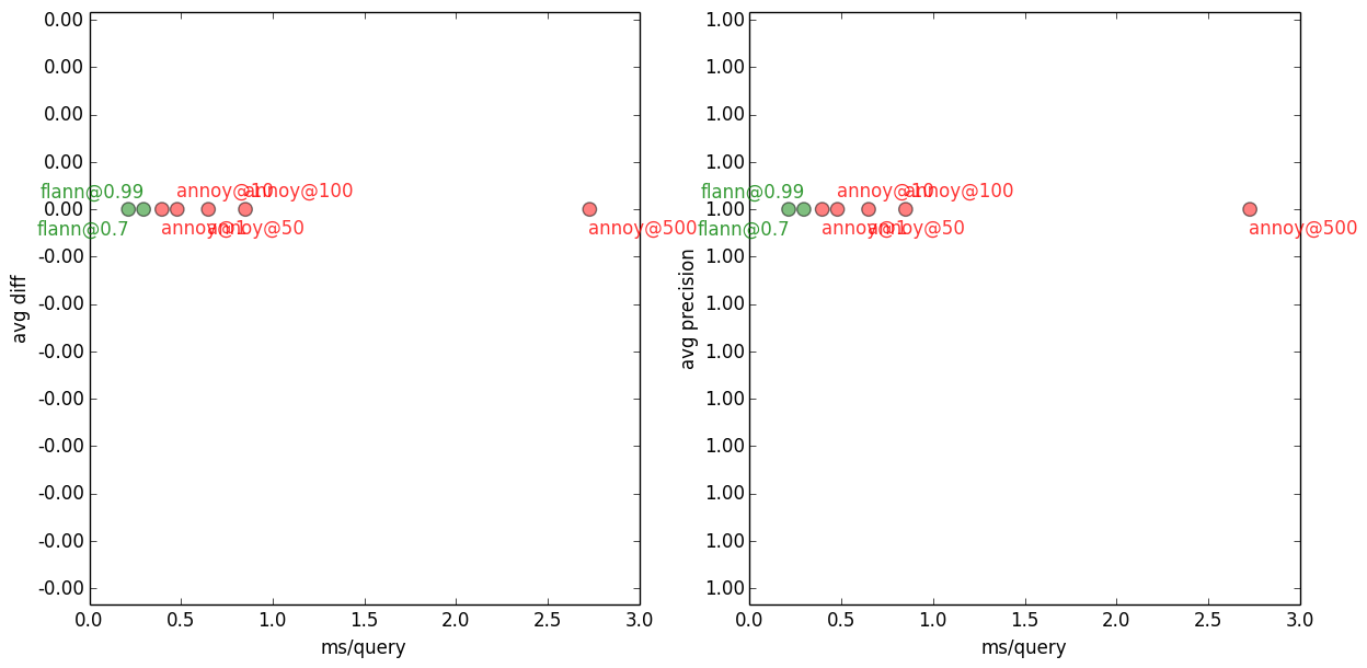
10-NN FLANN avg error vs. speed (left) and precision vs. speed (right), for several FLANN accuracy settings. All measurements are an average over 100 (distinct) queries. Each reported timing is the best of three runs, using a single core, on a dedicated Hetzner EX40-SSD machine.
For example, when the FLANN index is built with target_precision=0.7, getting top-10 nearest neighbours to a query takes ~0.26ms (wow!), but it gets only 2.3 out of 10 nearest neighbours right, on average. And cosine similarities of these FLANN neighbours are on average ~0.09 away from the “ideal” neighbour similarities. With FLANN index built at target_precision=0.99, the speed drops to ~0.33ms/query (still wow!), but average precision rises to ~0.37 and average error drops to ~0.04. Unsurprisingly, the greater the accuracy requested, the slower the query (and the larger the index).
Interestingly and annoyingly, the 0.04 (or 4%) average cossim error is the best FLANN can do, on this dataset. When asked to build a more accurate index, something inside FLANN overflows and indexing hangs in an infinite loop.
A few words on accuracy: as shown above, I recorded two different measures, each with a different focus. Precision is defined as the amount of overlap between retrieved documents and expected documents (=what an exact search would return). For example, if we ask an approximative method for the top-3 most similar documents, and it returns [doc_id1, doc_id2, doc_id3], while the exact three nearest neighbours are [doc_id2, doc_id3, doc_id4], the precision will be 2/3=0.67. Precision is a number between 0.0 and 1.0, higher is better. The document order (ranking) doesn’t matter for this measure.
The other accuracy measure is average similarity difference (~regret on cumulative gain), which is the average error in cosine similarity, again measured between the approximate vs. exact results. Smaller is better. For the same example as above, if a method returns top-3 similarities of [0.98, 0.9, 0.7], and the exact top-3 similarities are [0.98, 0.94, 0.9], its avg diff will be ((0.98-0.98) + (0.94-0.9) + (0.9-0.7)) / 3 = 0.08. Again, the particular ranking of results makes no difference.
Average difference makes better sense than precision in exploratory apps, where we don’t care about what particular documents are retrieved, as long as they are all as similar to the query as possible. I picked avg error because it’s intuitive and makes the accuracy results easy to interpret and reason about. More refined extensions, like the (normalized) discounted cumulative gain, exist and can be tuned in retrieval apps. I also recorded std dev and max of the errors, you can find them in the table at the end.
I won’t be going over the library or dataset descriptions here again; see the previous post for that.
Comparisons
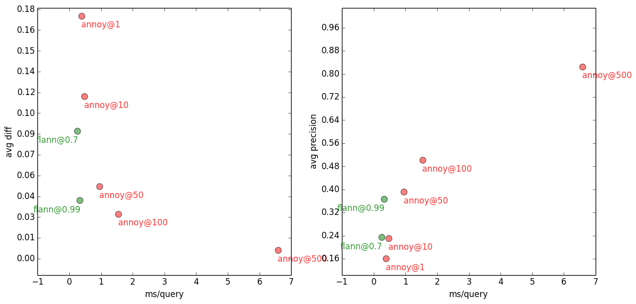
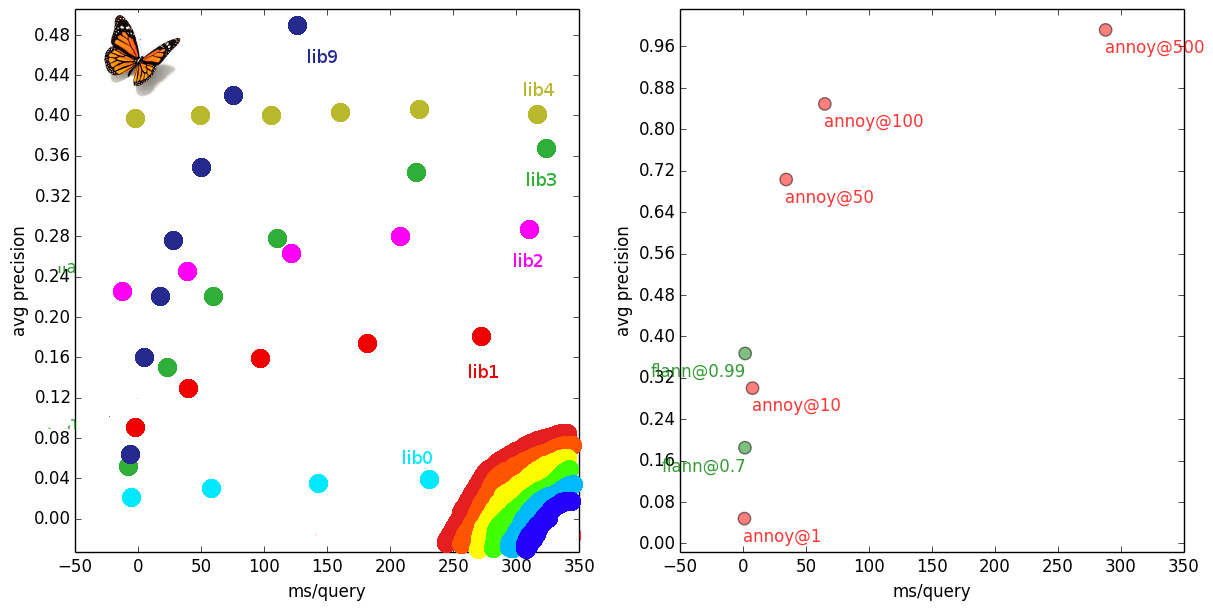
10-NN with Flann vs Annoy, on several accuracy settings.
It’s hard to tell from this graph, with the sub-millisecond values, but compared to FLANN, Annoy is about 4x slower on ± same accuracy. But unlike FLANN, Annoy has no problem getting arbitrarily close to the “exact” results. Annoy 10-NN gets to a respectable precision of 0.82 and avg error of 0.006 with only 6.6ms/query — see annoy@500 in the plots above. Compare that with gensim’s brute force search taking 679ms/query (precision 1.0, avg error 0.0) = ~100x slower than Annoy.
Scikit-learn manages to create an index (but not store it) before running out of RAM, on the 32GB Hetzner machine. Getting the 10 nearest neighbours takes 2143ms/query, neighbours are exact (precision 1.0, avg error 0.0). This is even slower than brute force search, so I removed scikit-learn from the contestants pool. To be fair, scikit-learn’s documentation hints that its algorithm is not likely to perform well in high dimensional spaces.
The following plots show the same comparison, but asking for a different number of “nearest neighbours”. For example, an application may be interested in only a single nearest neighbour. Or it may need 1,000 nearest neighbours. How do the k-NN libraries scale with “k”?
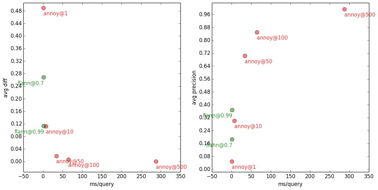
1000-NN with Flann and Annoy, on several accuracy settings.
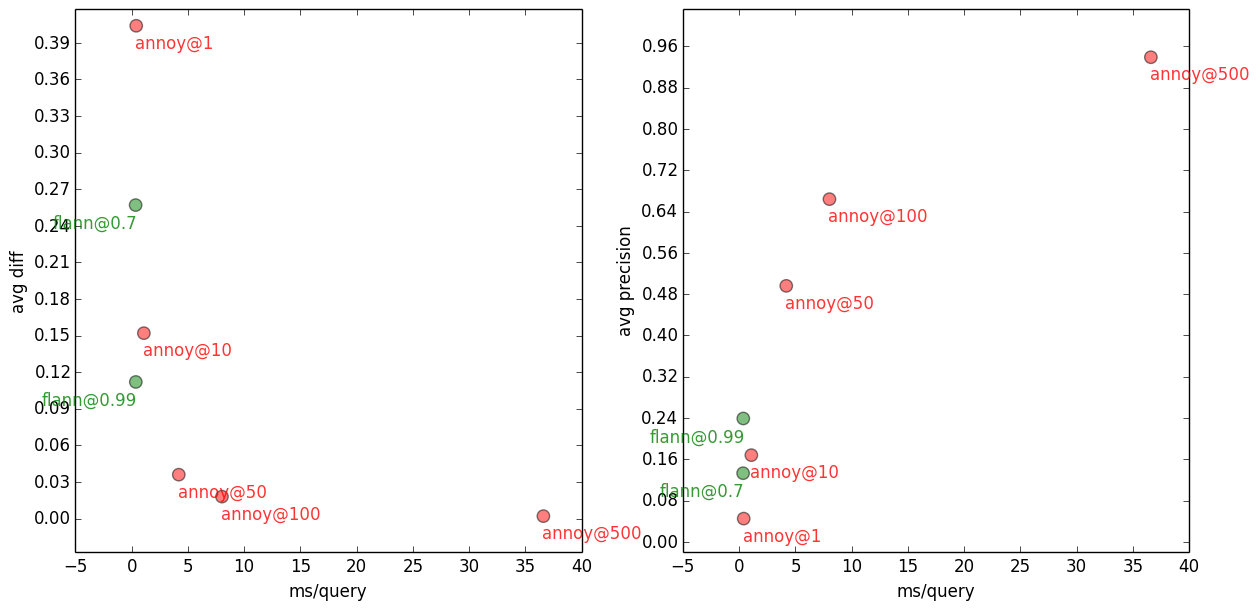
100-NN with Flann and Annoy, on several accuracy settings.
10-NN with Flann and Annoy, on several accuracy settings.
1-NN with Flann and Annoy, on several accuracy settings. All methods, on all settings, get the top one neighbour right, so it’s precision=1.0 and avgdiff=0.0 across the board.
Gensim (=brute force) doesn’t care about the number of neighbours, so its performance is 679ms/query regardless of “k”. When run in batch mode (issuing all 100 queries at once), average query time drops to 354ms/query.
In case you’re wondering where did the LSH contestant go: I didn’t manage to get LSH to behave nicely with regard to returning no less than “k” neighbours. I asked for top-10, got only 2 neighbours back and so on. Kind people pointed me toward NearPy, a much nicer implementation of LSH than Yahoo!’s. But even NearPy doesn’t solve the “k problem”. I opened a GitHub issue for this, your help is welcome! I’ll update the graphs with LSH measurements once they’re ready.
So, which nearest-neighbour implementation is the best?
FLANN is spectacularly fast, but it’s hard to say how it would fare on better accuracies.
On that note, let me say one more thing: getting to these results was about a hundred times more painful than I had anticipated. Lots of suffering. Things freezing, or not compiling, then compiling but failing tests, running out of memory, quirky idiosyncratic interfaces… And that’s not counting the libraries that I had pruned outright last time. I really thought the landscape of open source high-dim k-NN implementations would be a lot merrier than this. I find it surprising, given how fundamental and well-researched the domain is academically.
Landscape of open source high-dim similarity libraries for Python. Left: What I imagined. Right: Reality, one-and-a-half survivors. Brutal shootout.
Ok. So, each library takes a different approach, has different weak points, excels in different things. Results may vary with different datasets, yadda yadda. I hate vapid conclusions, so I’ll pick a winner anyway: the best implementation is Spotify’s Annoy.
FLANN is faster, but Annoy is saner. I like how it has a single parameter that controls accuracy that “just works”. It offers pleasant accuracy/speed tradeoffs, a responsive developer, is memory lean, concise, supports mmap for sharing an index between processes (FLANN can only share the input matrix, and not the index itself).
So I’ll probably plug either Annoy or NearPy into gensim, depending on how the “k” thing in LSH pans out. I’d likely reimplement Annoy in NumPy anyway though, because Annoy’s dependency on a C++ compiler and Boost is annoying (ha!), going against gensim’s “for humans” goal.
Bonus application
A bonus app for those who managed to read this far: type a title of any Wikipedia article exactly as it appears on Wikipedia, including letter casing, and see what the top-10 most similar articles are:
{{1000*result.taken|number:0}}ms; top10: {{result.nn}}
This uses the annoy@100 index (average precision 50%, average similarity error 3%) over all ~3.5 million LSI vectors (=Wikipedia documents). Mind that this is only a performance/sanity check; there was no quality tuning nor NLP preprocessing done to the Wikipedia corpus.
Appendix: Raw measurements & code
Measurements in table form, including how large the various indexes were when serialized to disk:| library@settings | k | prec | avg diff | std diff | max diff | query [ms] | index size [GB] | mmap'able portion of index [GB] |
|---|---|---|---|---|---|---|---|---|
| gensim@openblas | any | 1.00 | 0.00 | 0.000 | 0.00 | 678.9 | 6.6 | 6.6 |
| annoy@1 | 1 | 1.00 | 0.00 | 0.000 | 0.00 | 0.4 | 6.7 | 6.7 |
| annoy@10 | 1 | 1.00 | 0.00 | 0.000 | 0.00 | 0.5 | 7.1 | 7.1 |
| annoy@50 | 1 | 1.00 | 0.00 | 0.000 | 0.00 | 0.6 | 8.8 | 8.8 |
| annoy@100 | 1 | 1.00 | 0.00 | 0.000 | 0.00 | 0.9 | 11.0 | 11.0 |
| annoy@500 | 1 | 1.00 | 0.00 | 0.000 | 0.00 | 2.7 | 29.0 | 29.0 |
| annoy@1 | 10 | 0.16 | 0.17 | 0.163 | 0.87 | 0.4 | 6.7 | 6.7 |
| annoy@10 | 10 | 0.23 | 0.12 | 0.126 | 0.55 | 0.5 | 7.1 | 7.1 |
| annoy@50 | 10 | 0.39 | 0.05 | 0.064 | 0.36 | 1.0 | 8.8 | 8.8 |
| annoy@100 | 10 | 0.50 | 0.03 | 0.043 | 0.19 | 1.6 | 11.0 | 11.0 |
| annoy@500 | 10 | 0.82 | 0.01 | 0.013 | 0.07 | 6.6 | 29.0 | 29.0 |
| annoy@1 | 100 | 0.04 | 0.40 | 0.225 | 0.87 | 0.4 | 6.7 | 6.7 |
| annoy@10 | 100 | 0.17 | 0.15 | 0.126 | 0.56 | 1.1 | 7.1 | 7.1 |
| annoy@50 | 100 | 0.50 | 0.04 | 0.039 | 0.21 | 4.2 | 8.8 | 8.8 |
| annoy@100 | 100 | 0.66 | 0.02 | 0.024 | 0.13 | 8.0 | 11.0 | 11.0 |
| annoy@500 | 100 | 0.94 | 0.00 | 0.005 | 0.07 | 36.6 | 29.0 | 29.0 |
| annoy@1 | 1000 | 0.05 | 0.49 | 0.193 | 0.93 | 1.0 | 6.7 | 6.7 |
| annoy@10 | 1000 | 0.30 | 0.11 | 0.085 | 0.48 | 7.4 | 7.1 | 7.1 |
| annoy@50 | 1000 | 0.70 | 0.02 | 0.020 | 0.11 | 34.2 | 8.8 | 8.8 |
| annoy@100 | 1000 | 0.85 | 0.01 | 0.010 | 0.10 | 64.8 | 11.0 | 11.0 |
| annoy@500 | 1000 | 0.99 | 0.00 | 0.001 | 0.01 | 287.7 | 29.0 | 29.0 |
| [email protected] | 1 | 1.00 | 0.00 | 0.000 | 0.00 | 0.2 | 6.8 | 6.6 |
| [email protected] | 1 | 1.00 | 0.00 | 0.000 | 0.00 | 0.3 | 10.0 | 6.6 |
| [email protected] | 1 | 1.00 | 0.00 | 0.000 | 0.00 | 0.3 | 10.0 | 6.6 |
| [email protected] | 10 | 0.23 | 0.09 | 0.112 | 0.83 | 0.3 | 6.8 | 6.6 |
| [email protected] | 10 | 0.35 | 0.04 | 0.053 | 0.71 | 0.3 | 10.0 | 6.6 |
| [email protected] | 10 | 0.37 | 0.04 | 0.048 | 0.27 | 0.3 | 10.0 | 6.6 |
| [email protected] | 100 | 0.13 | 0.26 | 0.212 | 0.91 | 0.3 | 6.8 | 6.6 |
| [email protected] | 100 | 0.25 | 0.12 | 0.114 | 0.82 | 0.4 | 10.0 | 6.6 |
| [email protected] | 100 | 0.24 | 0.11 | 0.100 | 0.87 | 0.4 | 10.0 | 6.6 |
| [email protected] | 1000 | 0.18 | 0.27 | 0.205 | 0.95 | 1.4 | 6.8 | 6.6 |
| [email protected] | 1000 | 0.33 | 0.13 | 0.127 | 0.78 | 1.6 | 10.0 | 6.6 |
| [email protected] | 1000 | 0.37 | 0.11 | 0.119 | 0.80 | 1.6 | 10.0 | 6.6 |
| scikit-learn@auto | 10 | 1.00 | 0.00 | 0.000 | 0.00 | 2142.8 | - | - |
By the way, I extended all the evaluation code so that running a single bash script will download the English wiki, parse its XML, compute the Latent Semantic vectors, create all indexes, measure all timings, flush the toilet and brush your teeth for you, automatically. You can find the repo on GitHub: https://github.com/piskvorky/sim-shootout.
(If you liked this series, you may also like Optimizing deep learning with word2vec.)

Comments 38
query:”gensim
7ms; top10: [“Gensim”,”Snippet (programming)”,”Prettyprint”,”Smalltalk”,”Plagiarism detection”,”D (programming language)”,”Falcon (programming language)”,”Intelligent code completion”,”OCaml”,”Explicit semantic analysis”]
Author
500 topics is not nearly enough to represent the entirety of human knowledge in Wikipedia… but it’s better than I expected 🙂
It might be worth computing cosine similarity directly on sparse vectors. Thus, 500-element dense vectors should be only use for a filtering stage. This was done by Petrovic et al (see below). Interestingly, they don’t use pure LSH. They also employ a small inverted index built over relatively few recent Twitter entries.
First Story Detection – Association for Computational Linguistics http://www.aclweb.org/anthology/N10-1021.pdf
Hi, yesterday I tweeted about this paper: http://www.cs.ucr.edu/~jzaka001/pdf/SearchingMiningTrillionTimeSeries.pdf
It’s for time series and dynamic time warping but I think that most of its ideas (mainly 4.2.2 and possibly 4.2.4) can be used even for exact nearest neighbour search.
Author
Hello Michal, interesting article!
4.2.2. would hurt cache locality, so I doubt it is useful for simple (fast) measures like euclidean/cosine similarity. Plus it increases the index size a lot (need to store the feature ordering for each datapoint).
4.2.4. I flirted with pruning by lower bounds a bit too, using Weber’s VA-files. If implemented right, I think it could speed up searches by a nice, fat constant factor. Plus it’s critical for datasets where the “full” index is too large for RAM while the “small index” would still fit.
Anyway I downloaded their “trillion” code, I’ll check it out in more detail later 🙂
Actually, it won’t be bad, if the size of the vector is 500. Even if you use a super-efficient C++ SIMD-vectorized implementation of the distance, it takes about 500 CPU cycles to compute the distance.
If the distance computation is not vectorized, it is 1500 CPU cycles.
At the same time, a cache miss costs you no more than 230 CPU cycles on modern platforms. So, more efficient early termination technique can easily outstrip disadvantages of non-locality.
Even if non-locality is an issue, you can use bucketing. Essentially, you can group a few records and compute distances in batches.
Author
Hello Leo — that’s one miss *per feature*, while still assuming accessing the indices themselves comes for free. Could be avoided with clever prefetching, I suppose. Or perhaps indexing the vectors in sorted order makes more sense — only the query will be random accesses, and query can be cached entirely.
Ten years ago, I would have jumped at such an implementation eagerly 🙂 Maybe on a lonely weekend…
Bucketing is an interesting idea too.
I don’t see how it is one miss per feature. It is one miss per vector. At least in C++, vector elements are stored contiguously in memory.
Author
Unless I misunderstood it, the optimization in 4.2.2 accesses indexed vector elements out of order. The order is given by feature indices that will sort the query elements into descending order.
Ok, I, perhaps, need to study this paper in more detail.
since the 1NN is the query document itself, you should always query +1 objects.
As for LSH, it cannot guarantee to find k neighbors. When the hash bins contain less than k objects, what are you going to do? Even with a well-tuned multiprobe strategy, you will have sometimes too few candidates.
you may want to give m-trees and egress a try, but I don’t know if there’s a good Python implementation. maybe try the ball-tree though.
Author
1. 1NN: that’s on purpose
2. LSH: maybe tune larger (~large enough for “k”) bins, see the linked NearPy ticket
3. scikit-learn uses ball-tree
If you find more/better implementations you can try them, the benchmark code is public, let me know.
Thanks Radim for these 2 blog entries! Very interesting benchmark!
Nice blog post (series), Radim! Very interesting! 😉
Author
My pleasure meneer 🙂
Just released my K-NN search library at kgraph.org. I think my library will beat all the methods you tried.
Author
Do you have python wrappers? No need to “think”, we can run the benchmark and know for certain how your library compares on large datasets 🙂
Radim,
There do appear to be python bindings for kgraph,
http://www.kgraph.org/index.php?n=Main.Python
Ahoy Radime.
very instructive post. Thank you for performing this careful work. One thing you don’t mention, is radius-neighbor search. For some machine learning applications, one needs all the neighbors (approximately) in a given radius R. I assume you did not do it. Do you know of any benchmarks for this task?
Author
Ahoj mmp — and thanks!
I don’t know of good benchmarks (beyond what a google search would yield you), sorry.
But please do post here if you find something. Radius queries are very useful and a large research domain again, I’d be interested in a followup.
Thanks for writing this! Saved me a lot of time.
Great series Radim, very informative and well written. Many thanks for this.
At the end of this post you wrote “I’d likely reimplement Annoy in NumPy”. I was wondering if you had any success with this and if you were planning on sharing it.
I have also found the dependency of Annoy on a C compiler and Boost a freaking nightmare, specially for Windows (the latter might be more the problem though, not the dependency itself).
Did you run your Wiki test on NearPy,and if so, how did it compare to Flann and Annoy?
Author
Hello David, thanks 🙂
My gensim time is consumed by reviewing/cleaning up/merging other people’s contributions and pull requests lately. I don’t write that much code myself.
In short no, I haven’t re-implemented annoy yet. Do you want to try?
Hi Radim,
You might be interested in Maheshakya’s scikit learn GSOC project (Robert Layton and I are mentoring it); 4 weeks in, his implementation seems (on a particular benchmark) to dominate [1] Annoy on speed/precision and is close to FLANN’s speed. It is still early times, but your feedback is welcome.
[1] http://maheshakya.github.io/gsoc/2014/06/14/performance-evaluation-of-approximate-nearest-neighbor-search-implementations-part-2.html
Hi Radim, How long did it take you to build the index with annoy with 500 trees on the test set? I am trying to use annoy for a similar task, with 1.2 million nodes, 500-dim vectors, and 500 trees, but it seemed to take forever to build the index…
Author
Hello Xin, I checked the logs, and the annoy@500 index took 4h16m to build.
Thanks for this information!! I was using Euclidean distance. When I switched to Angular distance, I got at least 50x speed improvement on index building. And I should expected about the same speed as you had now.
I’m not too convinced by your results. I just used FLANN to NN with k-d trees. Insstead on automatically tuning parameters, I used 16 randomized trees and 8192 as checks for search parameters. With 500 nearest neighbors on a dataset of size 347,000 i got 86% precision for a query of size 10,000.
The automatic tuning didn’t work very well for me.
Author
Well, if you use a different dataset, different parameters and different evaluation criteria, you might get different results 🙂
I don’t think that’s very controversial.
Ahhh, apologies for making it sound controversial. That wasn’t my intention 😀 . Just wanted to confirm if you tried tweaking the parameters a bit or did you go with the autotuned parameters themselves ?
Author
Only to the degree described in the text of this blog series (`target_precision` etc).
Difficulty in setup / tuning internal parameters is actually one of the criteria on which I ultimately judged the libraries. Spending too much time on one library or another would beat the purpose.
Ultimately, the best library is the one you write yourself for your particular dataset and application (if you really want something super-tuned).
Pingback: (note (code cslai)) | Information Retrieving with ….. a lot of libraries
Hi Radim,
I just stumbled over this blog-entry while searching for similarity analysis stuff. Great stuff, thank you!!
Now the question is whether to use gensim or annoy: Basically, I don’t have a performance-issue, because I’m searching within a relatively small dataset (10,000 – 100,000 docs). I’m more interested in accuracy.
Do you think gensim alone would be enough in such a situation? Basically, the only thing I want to know is whether a doc (size: somewhere between 100-500 words) is similar to some of the 10,000 or 100,000 documents I have stored/indexed.
Author
Hello Imdat,
for small document collections, the linear bruteforce search will be blazingly fast and 100% accurate. And without the {technical, cognitive} overhead of the more complex approximative solutions.
Of course it depends on your other performance and concurrency requirements, but for 10k-100k docs, I wouldn’t bother with more complex algorithms.
Hope that helps!
HI Radim
So which algorithm did you finally implemented in Gensim? Annoy? Nearpy? Flann?
Does this mean that gensim already has the best nearest neighbour search ? Can you point me to which library it is? and how can we handle a case where we need online addition of vectors to the index + persistent storage of the index?
Author
In the end we added integration with Annoy to gensim.
But if you need online addition of new vectors, use the Similarity class instead. Annoy doesn’t support it.Similarity has persistent storage of the index too (using sharding).
Pingback: Concept Search on Wikipedia - Nearist
I’ve used gensim word2vec to train my large dataset and when i searched a word “mutation” as model.most_similar(“mutation”) it gives an error as “word” not present in vocabulary. How I can add new word into my exisiting vocab so that I can get its vector array and most similar words around it??